How to average multiple vlookup findings in Excel?
In many practical situations, a lookup value might appear multiple times within your table, and each occurrence may have an associated value that you wish to include in your calculations. If you need to calculate the average of all values that match a particular lookup value—essentially averaging the results of multiple vlookup matches—Excel offers several methods to accomplish this efficiently. By averaging all target values matching a lookup value, you can gain deeper insights for tasks such as sales analysis, quality control, or summarizing survey results. In this comprehensive article, you will find clear instructions for a range of solutions, from formula-based approaches to advanced tools, along with their scenarios, strengths, and limitations.
- Average multiple vlookup findings with formula
- Average multiple vlookup findings with Filter feature
- Average multiple vlookup findings with Kutools for Excel
- Average multiple vlookup findings with Pivot Table
- Average multiple vlookup findings with VBA macro
Average multiple vlookup findings with formula
When you need to find and average several values associated with the same lookup item, using a direct formula is one of the fastest and most flexible ways. The AVERAGEIF or an array formula handles this easily without creating extra columns.
Enter the following formula in a blank cell (for example, F2):
=AVERAGEIF(A1:A24,E2,C1:C24)Press the Enter key after typing the formula. This immediately gives you the average of all values in column C where the corresponding value in column A matches your lookup value located in cell E2. See the illustration below:
Parameter explanation and tips:
- A1:A24: The range containing your lookup values.
- E2: The specific value you want to look up.
- C1:C24: The range from which you want to average the matching values.
Alternative approach (for users comfortable with array formulas):
Enter the following formula in a blank cell and use Ctrl + Shift + Enter to confirm:
=AVERAGE(IF(A1:A24=E2,C1:C24))Array formulas process each comparison individually, which is helpful in versions of Excel that do not support dynamic arrays. Carefully ensure the ranges are exactly the same size to avoid errors.
Practical scenarios and notes:
- Best for datasets that are not filtered and have straightforward lookup needs.
- If either range includes empty cells, those are ignored in the average calculation.
- In dynamic tables or when adding data, consider using table references for more robust formulas.
- Watch out for accidental mismatches of cell ranges, which are a common source of incorrect averages or errors.
Average multiple vlookup findings with Filter feature
The Filter function in Excel allows you to temporarily hide rows that do not meet specific criteria, making it easier to focus on the results you need. This technique enables you to isolate all records matching your lookup value and then quickly calculate the average value of the visible entries.
1. Select the header row of your data, then navigate to Data > Filter. /p>
/p>
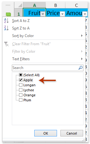
2. In the column containing the lookup values, click the filter drop-down arrow and select only the item you want to examine. Click OK to apply the filter. The table will then show only entries matching your lookup value. See the screenshot on the left:
3. Enter the following formula in a blank cell (such as below your data):
=AVERAGEVISIBLE(C2:C22)Press Enter to calculate the average of all currently visible (filtered) cells in column C. This ensures only the values displayed after filtering are included in the result.
Advantages and scenarios: This approach is ideal when you want to manually inspect or process data interactively and your data is already arranged in a table with headers. It’s especially effective when working with complex filters or conditional formatting.
Limitations: If you modify or remove filters, the formula will adjust to whatever data is visible, and you need Kutools for Excel for the AVERAGEVISIBLE function (standard Excel does not have this function). Also, ensure no hidden rows unrelated to filtering are present, as those will also be excluded.
Demo: Average multiple vlookup findings with Filter feature
Average multiple vlookup findings with Kutools for Excel
If you often need to summarize and aggregate data based on duplicates, Kutools for Excel provides a practical solution through its Advanced Combine Rows utility. This tool can quickly combine or calculate values such as the average, sum, or count for matching records in one step, making it highly suitable for larger datasets or regular reports.
1. Highlight the range of your data table, including both the lookup column and the values to average. Then go to Kutools > Content > Advanced Combine Rows. See the screenshot:
2. In the dialog box that appears:
- Select the column with your lookup values and click Primary Key.
- Choose the column with your target values, then click Calculate > Average.
- Set combination or calculation rules for other columns as needed—such as combining text with commas or applying sum, max, or min.
3. Click Ok to apply the settings.
The rows with duplicate lookup values are now merged, and the values in the designated column are automatically averaged for every unique lookup value. This is particularly helpful for preparing summary reports or condensing data.
Practical tip: Using Advanced Combine Rows minimizes manual calculation and potential for mistake. The tool is best for users who regularly process data with recurring lookup values and want actionable summaries quickly. Always double-check that the correct columns are assigned before combining, especially if data structure changes.
Kutools for Excel - Supercharge Excel with over 300 essential tools. Enjoy permanently free AI features! Get It Now
Demo: average multiple vlookup findings with Kutools for Excel
Average multiple vlookup findings with Pivot Table
Pivot Tables offer a dynamic and visual approach to summarizing and analyzing data. Using a Pivot Table, you can automatically group entries by their lookup value and display the average of a target column for each group, providing an interactive summary that updates as your data changes.
Most effective scenarios: This approach is well suited when you need an overall summary for all lookup values at once, rather than focusing on a single lookup value. Pivot Tables are also excellent for quick data exploration, report generation, and when you wish to present your results in a sortable, expandable format.
Instructions:
- Select your entire dataset, including headers.
- Go to Insert > PivotTable > From Table or Range. Choose to place the Pivot Table on a new worksheet or an existing one as needed.
- In the PivotTable Fields panel, drag the column containing your lookup values into the Rows area.
- Drag the column you want to average into the Values area. Click the value field, select Value Field Settings, then set the calculation type to Average.
This results in a summary table listing each unique lookup value with its average calculated for the associated data. You can easily change grouping, filter, or drill down to details as needed.
Pros: No formulas required, supports dynamic updates, suitable for reporting and data exploration.
Cons: Extra steps needed to refresh after data changes, less suitable for extracting a single value directly into other formulas, and initial setup requires basic familiarity with PivotTables.
Troubleshooting tips: If values appear as counts or sums instead of averages, check the field calculation setting. For best results, ensure columns have appropriate headings and clarify any duplicated column names before creating the Pivot Table.
Average multiple vlookup findings with VBA macro
For advanced users and those managing data that updates regularly, using a VBA macro allows for automation of the averaging process across all entries matching a lookup value. This method loops through your data to find every match and computes the average, making it suitable for large datasets or when you need a repeatable workflow.
Applicable scenarios and notes: VBA is ideal when you frequently need to perform the average calculation, want to automate reports, or require a flexible approach that can be tailored to unusual data layouts. VBA macros work best when you are comfortable enabling macros in your workbook and require custom outputs.
1. Go to the Developer tab, choose Visual Basic or press Alt + F11 keys to open the VBA editor, then click Insert > Module. Copy and paste the code below into the new module:
Sub AverageVlookupMatches()
    Dim lookupCol As Range
    Dim avgCol As Range
    Dim lookupValue As Variant
    Dim total As Double
    Dim count As Long
    Dim i As Long

    On Error Resume Next
    xTitleId = "KutoolsforExcel"

    Set lookupCol = Application.InputBox("Select the lookup column", xTitleId, Selection.Address, Type:=8)
    Set avgCol = Application.InputBox("Select the column to average", xTitleId, , Type:=8)
    lookupValue = Application.InputBox("Enter lookup value", xTitleId, , Type:=2)

    Application.ScreenUpdating = False
    total = 0
    count = 0

    For i = 1 To lookupCol.Rows.Count
        If lookupCol.Cells(i, 1).Value = lookupValue Then
            If IsNumeric(avgCol.Cells(i, 1).Value) Then
                total = total + avgCol.Cells(i, 1).Value
                count = count + 1
            End If
        End If
    Next i

    If count > 0 Then
        MsgBox "Average of all matches: " & total / count, vbInformation, "Result"
    Else
        MsgBox "No matches found.", vbExclamation, "Result"
    End If

    Application.ScreenUpdating = True
End Sub
2. After pasting the code, close the VBA editor. To run the macro, return to Excel, press the F5 key, or click Run. When prompted, select the lookup column, the value column to be averaged, and enter the lookup value. The macro will display the calculated average in a message box.
Practical tips and precautions: Make sure your lookup and value columns have the same number of rows, and there are no blank rows within the selected areas. Entries with non-numeric values in the target column will be ignored. For best automation, adjust named ranges or macro logic as necessary to your worksheet layout.
Troubleshooting: If you encounter "No matches found," check for leading/trailing spaces or data type inconsistencies in your lookup column. Ensure macros are enabled for execution.
Related articles:
Calculate average/compound annual growth rate in Excel
Calculate moving/rolling average Excel
Average per day/month/quarter/hour with pivot table in Excel
Best Office Productivity Tools
Supercharge Your Excel Skills with Kutools for Excel, and Experience Efficiency Like Never Before. Kutools for Excel Offers Over 300 Advanced Features to Boost Productivity and Save Time. Click Here to Get The Feature You Need The Most...
Office Tab Brings Tabbed interface to Office, and Make Your Work Much Easier
- Enable tabbed editing and reading in Word, Excel, PowerPoint, Publisher, Access, Visio and Project.
- Open and create multiple documents in new tabs of the same window, rather than in new windows.
- Increases your productivity by 50%, and reduces hundreds of mouse clicks for you every day!
All Kutools add-ins. One installer
Kutools for Office suite bundles add-ins for Excel, Word, Outlook & PowerPoint plus Office Tab Pro, which is ideal for teams working across Office apps.
- All-in-one suite — Excel, Word, Outlook & PowerPoint add-ins + Office Tab Pro
- One installer, one license — set up in minutes (MSI-ready)
- Works better together — streamlined productivity across Office apps
- 30-day full-featured trial — no registration, no credit card
- Best value — save vs buying individual add-in