How to conditional formatting based on another sheet in Google sheet?
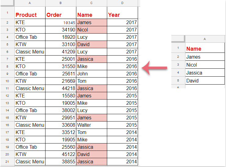
Conditional formatting is a useful feature in Google Sheets that allows you to automatically highlight cells based on specific criteria, making it easier to analyze and visualize your data. Sometimes, instead of highlighting cells according to values within the same sheet, you may need to base your formatting rules on a reference list or criteria stored in a different sheet. For example, you might want to highlight cells in one sheet that also appear in a list maintained in another sheet, as illustrated in the screenshot below. This kind of task is common when you are working with cross-referenced data, such as comparing current sales to a master product list, or checking for duplicate entries against another data source. However, setting up such conditional formatting in Google Sheets—especially when referencing data across sheets—can be confusing if you haven’t done it before. The guide below will show you, step-by-step, a straightforward approach to accomplish this.
Conditional formatting to highlight cells based on a list from another sheet in Google Sheets
Conditional formatting to highlight cells based on a list from another sheet in Google Sheets
This method lets you set up a conditional format rule to highlight cells in your active sheet if they appear in a specified list from another sheet. Such cross-sheet conditional formatting is particularly useful for dynamic data monitoring and maintaining consistency between related datasets.
To complete this process, follow these detailed steps:
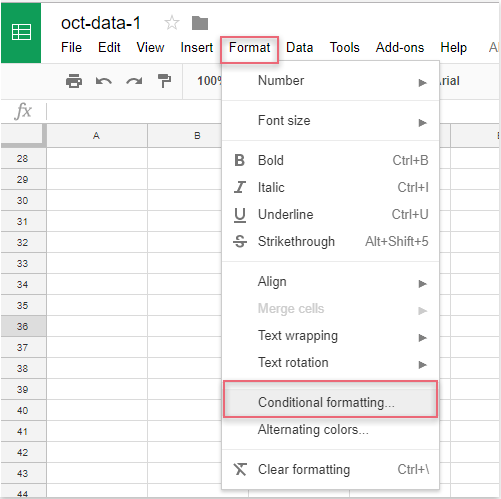
1. Open your target worksheet, then click the Format menu at the top, and select Conditional formatting. The Conditional format rules pane will open on the right side of your screen.
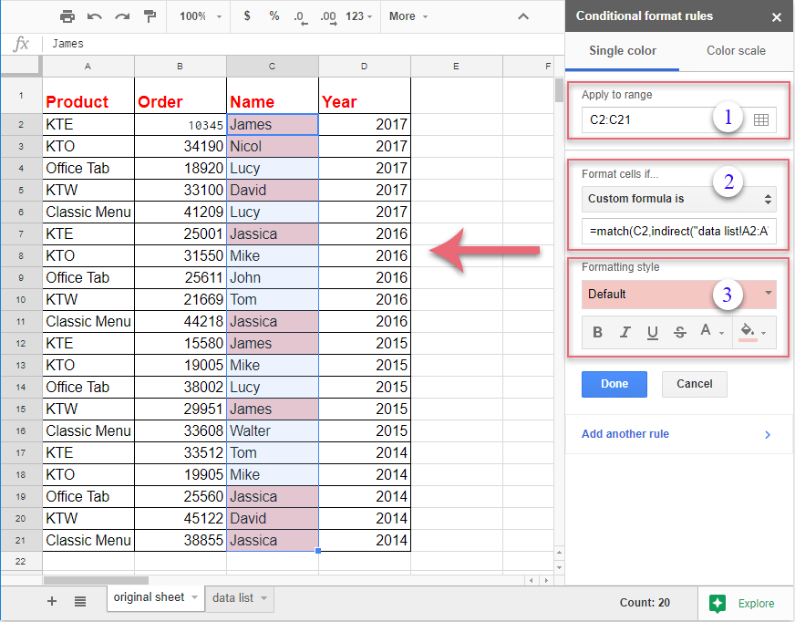
2. On the Conditional format rules panel, take the following actions:
(1.) Click the ![]() button next to the "Apply to range" field. Select the range of cells you wish to highlight. For example, if you want to format all the values in column C from row 2 downwards, select C2:C. Selecting an appropriate range ensures only the intended cells are evaluated for formatting.
button next to the "Apply to range" field. Select the range of cells you wish to highlight. For example, if you want to format all the values in column C from row 2 downwards, select C2:C. Selecting an appropriate range ensures only the intended cells are evaluated for formatting.
(2.) In the Format cells if drop-down menu, choose Custom formula is. Enter the following formula into the provided box:=match(C2,indirect("data list!A2:A"),0). This formula checks whether each cell in column C matches any value in the range A2:A of the "data list" sheet.
(3.) Under Formatting style, select your desired formatting, such as filling the cell with a specific color or changing the font style. You can preview the style immediately in your sheet before applying it.
Note: In the above formula, C2 refers to the first cell in your selected range (adjust if your data starts in a different row or column), and data list!A2:A refers to the sheet name (“data list”) and the corresponding range (A2:A) where your list from another sheet is stored. Make sure the cell reference in the formula matches the top-left cell of your selected range, otherwise the formatting may not apply correctly. If your data list range is different, remember to update it in the formula (for example, “data list!B2:B”).
3. Once you have set up the rule, matching cells in your chosen range will be instantly highlighted based on the list from the other sheet. Review the preview, then click Done at the bottom of the Conditional format rules pane to apply and save your formatting.
Tips and troubleshooting:
- Double-check for typographical errors in your formula, especially in sheet names and range references—incorrect references are a common reason rules fail to apply.
- If your data list contains blank cells, the
MATCHfunction will return an#N/Aerror for non-matching values, but this is expected behavior and does not affect the highlighting of matching items. - When you copy formatting to a new sheet or adjust ranges, ensure you also update the cell references in your custom formula accordingly.
- The formatting updates automatically if you later add or remove items from your reference list.
- The sheet and range referenced in your formula exist and are spelled correctly.
- The first cell in your formula matches the first cell of your selected range.
- All needed permissions for cross-sheet access within your spreadsheet are available—this method works within a single multi-sheet Google Sheets file, not across different files.
As an alternative, if your data structure or requirements are more complex—for example, if you need to compare multiple columns, allow for partial matches, or perform more advanced lookups—using helper columns with COUNTIF or VLOOKUP formulas, or employing Google Apps Script (custom JavaScript code), can also achieve flexible conditional formatting solutions.
In summary, setting up conditional formatting based on another sheet is highly effective for list checking, duplicate tracking, and various cross-sheet data validations—all within Google Sheets. Always confirm your formula inputs, reference ranges, and formatting rules for smooth and accurate results.

Unlock Excel Magic with Kutools AI
- Smart Execution: Perform cell operations, analyze data, and create charts—all driven by simple commands.
- Custom Formulas: Generate tailored formulas to streamline your workflows.
- VBA Coding: Write and implement VBA code effortlessly.
- Formula Interpretation: Understand complex formulas with ease.
- Text Translation: Break language barriers within your spreadsheets.
Best Office Productivity Tools
Supercharge Your Excel Skills with Kutools for Excel, and Experience Efficiency Like Never Before. Kutools for Excel Offers Over 300 Advanced Features to Boost Productivity and Save Time. Click Here to Get The Feature You Need The Most...
Office Tab Brings Tabbed interface to Office, and Make Your Work Much Easier
- Enable tabbed editing and reading in Word, Excel, PowerPoint, Publisher, Access, Visio and Project.
- Open and create multiple documents in new tabs of the same window, rather than in new windows.
- Increases your productivity by 50%, and reduces hundreds of mouse clicks for you every day!
All Kutools add-ins. One installer
Kutools for Office suite bundles add-ins for Excel, Word, Outlook & PowerPoint plus Office Tab Pro, which is ideal for teams working across Office apps.
- All-in-one suite — Excel, Word, Outlook & PowerPoint add-ins + Office Tab Pro
- One installer, one license — set up in minutes (MSI-ready)
- Works better together — streamlined productivity across Office apps
- 30-day full-featured trial — no registration, no credit card
- Best value — save vs buying individual add-in